Simulations of Evolutionary Games in Space
Hanjie Luo
School of Electronic and Computer Science
University of Southampton
6 February, 2011
Introduction
The basic rules of evolutionary games
Evolution of cooperative behaviour is widely existent in the biological organisms and social systems. In order to research the evolution of cooperation, some classical evolutionary games have been used, and Prisoners’ Dilemma (PD) is one of the famous models.
In this paper, I use a simplified version of Prisoners Dilemma which is played by two kinds of plays: those who always apply cooperation strategy, C, and those who always apply defection strategy, D, on a two-dimensional, n×n lattice with fixed boundary conditions. Each position is only occupied by a C or a D. The payoff matrix which describes the interaction is as follows:
1 | C D |
where, b is the only parameter which represents the advantage for defectors. In each generation of the game, each site-owner receives a score which is the sum of the pay-offs with 8 immediate neighbours and itself. In the next generation, each lattice-site is replaced by the highest-scoring player among 8 immediate neighbours and itself. I also explored the game played with only 8 immediate neighbours without self-interaction and 4 orthogonal neighbours with self-interaction.
Consequently, different chaotically changing patterns can be generated by setting different initial condition and different regimes of parameter b. Nowak and May observed that \(2>b>1.8\) is the most significant regime where C and D both will grow which makes the frequency of cooperators always reaches approximately 0.318 regardless of initial conditions (1992: 826).
As an extension, I study the evolutionary game in three-dimensional space and predict that it has the same performance as the game in two-dimensional space.
Reimplemented Results
8-neighbours with self-interaction
Figure 1 shows two different asymptotic patterns which are generated by PD for two different magnitude ob b. for \(1.75<b<1.8\), D clusters will shrink while C will continue to grow. In this situation, figure 1a and 1b show that some D line fragments exist on the background of C. Figure 1c and 1d are for the significant regime \(1.8<b<2\) where C and D both persist in expending thereby creating the chaotic dynamic patterns. However, figure 2 shows that the frequency of cooperators \({f_c}\) is completely independent of all the starting conditions, which is around \(12\log 2 - 8 = 0.318\) (Nowak and May 1992: 826). It seems that there is a universal constant hiding in the PD.
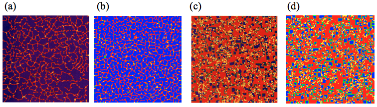
Figure 1. These figures are the patterns which are generated by Prisoners’ Dilemma for different magnitude of b. (a) and (c) are the original pictures from paper while (b) and (d) are reimplemented figures. All simulations start with the initial condition with 10% defectors at a 200×200 square-lattice with fixed boundary conditions. The figures show the generation \(t>100\). The colour coding is as follows: blue, a C site which was a C in the previous generation; red, a D site which was D; yellow, a D following a C; green, a C following a D. (a) and (b) are the patterns when \(1.75<b<1.8\) whereas (c) and (d) are the patterns when \(1.8<b<2\). (Nowak and May 1992: 827)
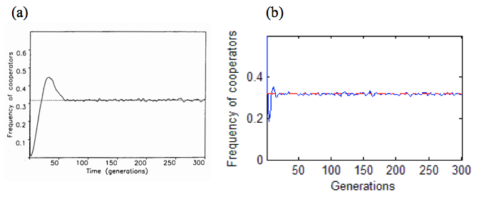
Figure 2. The frequency of cooperators with random initial conditions. (a) is the original figure from paper while (b) is reimplemented figure. The dashed or red line represents \({f_c=0.318}\). Conditions: 400×400 square lattice with fixed boundaries conditions, 8 neighbours plus self-interaction, \({f_c(0)=0.6}\), \(1.8<b<2\), 300 generations. (Nowak and May 1992: 827)
8-neighbours without self-interaction
A similar result was obtained by excluding self-interaction. However, there is a small different on the regimes of b values. The C clusters will continue to grow when \(b<5/3\) while D clusters will keep growing when \(b>8/5\). As a result, the most significant region is \(8/5<b<5/3\) where both C and D will continue to grow (Nowak and May 1992: 57). Figure 3a shows a symmetric pattern which starts from a single D at the centre of Cs. Figure 3b reveals that the frequency will converge to around 0.300 for random starting conditions, which is slight different from figure 2.
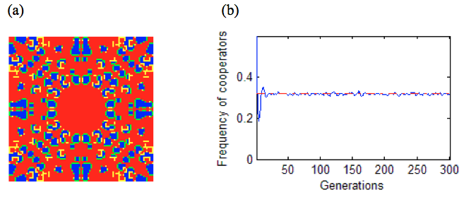
Figure 3. (a) The symmetric pattern generated by the evolutionary games. It begins with a single D at the centre of a 99×99 square lattice of Cs with fixed boundary conditions. Other conditions: 8-neighbours without self-interaction, \(8/5<b<5/3\), generations=218. (b) The frequency of cooperators for a 400×400 square lattice with fixed boundaries conditions, random initial conditions (10% defectors), \(8/5<b<5/3\), generations=300. The red line represents 0.300.
4-neighbours with self-interaction
The game played with 4 orthogonal neighbours plus self-interaction is also explored. The interesting regime has become \(5/3<b<2\) (Nowak and May 1992: 829). Figure 4a shows a different complex pattern contrasting with figure 3a. Similarly, figure 4b manifests that the frequency will converge to around 0.376 for random starting conditions.
By observing through figure 2, figure 3b and figure 4b, the frequency of cooperators always converge to a specific proportion. So, it seems that the results of the evolutionary games have some kind of robustness.
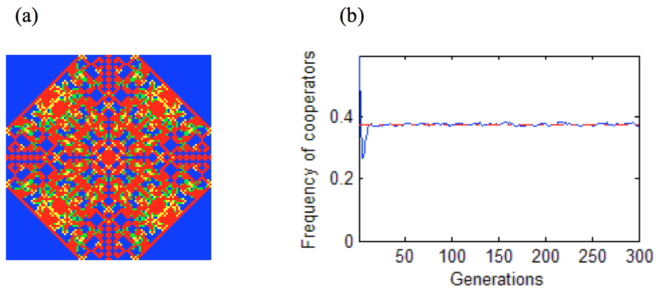
Figure 4. (a) The symmetric pattern of a square-lattice with 4 neighbours plus self-interaction which begins with a single D at the centre of a 99×99 square lattice of Cs with fixed boundary conditions, \(5/3<b<2\), generations=218. (b) The frequency of cooperators for a 400×400 square lattice with fixed boundaries conditions, random initial conditions (10% defectors), \(5/3<b<2\), generations=300. The red line represents 0.376.
Extensions
Evolutionary games in three dimensions
Introduction
The evolutionary games above are all played in two dimensions. So, it is interesting to study the evolutionary games in three dimensions and see what difference it makes contrasting to the games in two dimensions.
The basic rules are almost the same as two-dimensionl versions except the players are placed on an n×n×n cubic world. The interaction of the games is with the 26 immediate neighbours plus self-interaction.
The purpose of PD is to simulate the cooperate behaviors among biological organisms and social systems in the real world. However, the world we lived in is three-dimensional. Consequently, it is necessary to simulate in three dimensions for reaching valid results about real world. It is reasonable to forecast that the results of the games in three dimensions are very similar to the games in two dimensions which can also generate the symmetric patterns and the frequency will converge to a specified value because these results are widely seen in the games in two dimensions.
Results of extension
By experiment, I find that if \(b>1.421\), a 2×2×2 cube of D will keep growing at the corners while a 2×2×2 cube of C will keep expanding if \(b<2\). So the interesting regime has become \(1.421<b<2\) where both C and D will keep growing. Figure 5 shows different patterns for two different regimes of b values which both started with a single D at the centre Cs. For \(1.421<b<1.5\), I find symmetric patterns emerged while the patterns have become chaotic if \(1.5<b<2\), which is slight different from games played in two dimensions. Figure 6 shows that the frequency will converge to around 0.535 for all random starting conditions.
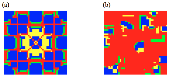
Figure 5. The patterns generated by PD in three dimensions. The games are played in a 45×45×45 cube with fixed boundary conditions. The interaction of the games is with the 26 immediate neighbours plus self-interaction. Both figures show a middle slice, 150 generations after having started with a single D at the centre Cs. (a) \(1.421<b<1.5\) (b) \(1.5<b<2\).
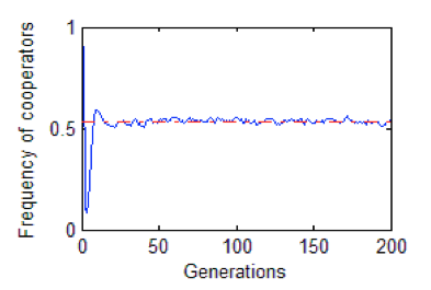
Figure 6. The frequency of cooperators for a 45×45×45 cube with fixed boundaries conditions, random initial conditions (10% defectors), \(1.421<b<2\), generations=200. The interaction of the games is with the 26 immediate neighbours plus self-interaction. The red line represents 0.535.
Conclusion
The results of simulations reveal that the PD in three dimensions has the same characteristics as the PD in two dimensions. As a result, we can use PD in two dimensions, which is less computing contrasting with PD in three dimensions, for simulating this three-dimensional real world.
Evolutionary games with asynchronous updating
Introduction
The rule described above means that all players are updated their states at the same time. However, a global clock which synchronizes their interactions is non-existent in a natural system. Consequently, it is necessary to update the states continuously and asynchronously for simulating a real world system (Huberman and Glance 1993: 7717).
In order to realize asynchronous updating, a small enough interval of time, which makes at most one site-owner interactions within that time interval, is randomly chosen. The chosen site-owner interactions with its neighoubers (with or without self-interaction) and replaces its state immediately while other states of site-owners stay constant. Consequently, the environment of the world will be changed slightly and continuously at each time interval. This procedure will continue until all entities have been chosen once.
Results of extension
Figure 8 shows that a synchronously updated games starts with a single D at the centre of Cs. The array will be eventually full of Ds within 100 generations, which is quite different contrasting with the synchronous version.
However, the situations are quite different when the interaction is with 4 neighbours plus interaction. Figure 9a reveals that the frequency will converge to around 0.500 for random starting conditions (including a single D at the centre of Cs). Figures 9b shows a similar pattern comparing with figure 1a.
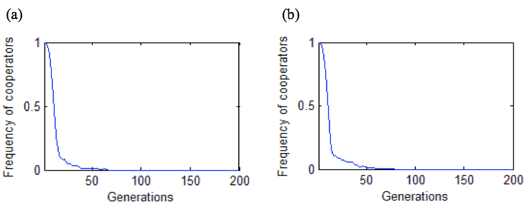
Figure 8. The frequency of cooperators with asynchronous updating. The games begin with a single D at the centre of a 99×99 square lattice of Cs with fixed boundary conditions. (a) Conditions: 8 neighbours plus self-interaction, \(1.8<b<2\). (b) Conditions: 8 neighbours exclude self-interaction, \(8/5<b<5/3\).
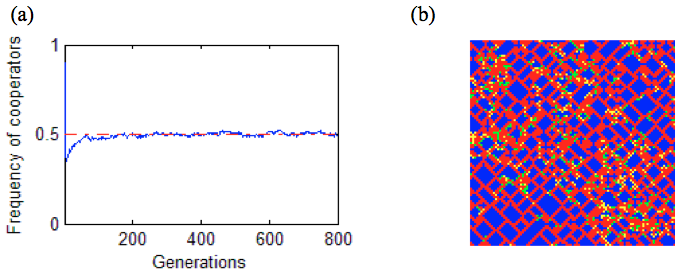
Figure 9. The results of PD with asynchronous updating. The games play at a 99×99 square lattice with fixed boundaries conditions, random initial conditions (10% defectors), \(5/3<B<2\), generations=800. (a) The frequency of cooperators. The red line represents 0.500. (b) The 800th generation of patterns.
Conclusion
The experiments show that, in an asynchronously updated game, the array will always be full of Ds as long as a C in the initial conditions when the interaction is with 8 neighbours with or without self-interaction. What’s more, I also find the frequency of cooperators always converge to a specific proportion if the interaction is with 4 neighbours plus self-interaction, which is the same characteristic occurring in synchronous version.
Recosures
References
Nowak, M, A and May, R, M 1992, ‘Evolutionary games and spatial chaos’, Nature, vol. 359, pp. 826-829.
Nowak, M, A and May, R, M 1993, ‘THE SPATIAL DILEMMAS OF EVOLUTION’, International Journal of Bifurcation and Chaos, vol. 3, no.1, pp. 35-78.
Huberman, B, A, and Glance, N, S, 1993, ‘Evolutionary games and computer simulations’, Proceedings of the National Academy of Sciences, vol. 90, no. 16, pp. 7716-7718.